6. 🧮 Leveraging video analytics (e.g., plots, etc)
In this section we show you how to create plots that show the exact moments (i.e., timestamps) in the video when a specific event happens.
We select the video we wish to analyze
dataset = tenyks.get_dataset("popeye")6.1 Plotting code (the MZ graph)
def convert_seconds(seconds):
    minutes = seconds // 60
    remaining_seconds = seconds % 60
return f"{minutes} minute(s) and {remaining_seconds} second(s)"import numpy as np
from datetime import timedelta
import pandas as pd
import matplotlib.pyplot as plt
def adjust_timestamp(row, part_durations):
part_index = row['video_key']
return row['timestamp'] + sum(part_durations[part] for part in part_durations if part < part_index)
def calculate_total_duration(clips):
return sum(clip.duration for clip in clips)
def merge_clips(clips):
sorted_clips = sorted(clips, key=lambda clip: (clip.video_key, clip.timestamp))
merged_clips = []
current_clip = None
for clip in sorted_clips:
if current_clip is None:
current_clip = clip
else:
current_end_time = current_clip.timestamp + current_clip.duration
new_clip_start_time = clip.timestamp
if current_clip.video_key == clip.video_key and current_end_time >= new_clip_start_time:
current_clip.duration = max(current_clip.duration, new_clip_start_time + clip.duration - current_clip.timestamp)
else:
merged_clips.append(current_clip)
current_clip = clip
if current_clip:
merged_clips.append(current_clip)
return merged_clips
def merge_intervals_and_calculate_duration(df):
merged_intervals = []
current_start, current_end = df.loc[0, 'adjusted_start'], df.loc[0, 'adjusted_end']
for i in range(1, len(df)):
start = df.loc[i, 'adjusted_start']
end = df.loc[i, 'adjusted_end']
if start <= current_end:
current_end = max(current_end, end)
else:
merged_intervals.append((current_start, current_end))
current_start, current_end = start, end
merged_intervals.append((current_start, current_end))
total_duration = sum(end - start for start, end in merged_intervals)
return total_duration, merged_intervals
def round_up_to_next_tick(value, tick_size):
"""Round up a value to the next multiple of tick_size."""
return np.ceil(value / tick_size) * tick_size
import numpy as np
from datetime import timedelta
import pandas as pd
import matplotlib.pyplot as plt
# Step 1: Function to generate the plot and return bars
def plot_histogram_and_return_bars(movie_title, part_durations, clips, search_term_label="Search Term", bin_size_minutes=10):
# First, merge the overlapping clips
merged_clips = merge_clips(clips)
# Create a DataFrame with the merged clips
df_clips = pd.DataFrame(
[{'video_key': clip.video_key, 'timestamp': clip.timestamp, 'duration': clip.duration} for clip in merged_clips])
# Adjust timestamps based on part durations
df_clips['adjusted_start'] = df_clips.apply(adjust_timestamp, axis=1, part_durations=part_durations)
df_clips['adjusted_end'] = df_clips['adjusted_start'] + df_clips['duration']
# Merge intervals and calculate the total duration
total_duration, merged_intervals = merge_intervals_and_calculate_duration(df_clips)
print(f"Total duration of {search_term_label} in \"{movie_title}\": {total_duration} seconds")
# Calculate movie duration and bin size in seconds
movie_duration = sum(part_durations.values())
bin_size_seconds = bin_size_minutes * 60
# Bin the merged intervals into bins of the specified size
bins = np.arange(0, movie_duration + bin_size_seconds, bin_size_seconds)
binned_durations = np.zeros(len(bins) - 1)
first_timestamps = [None] * (len(bins) - 1)
for start, end in merged_intervals:
for i in range(len(bins) - 1):
bin_start, bin_end = bins[i], bins[i + 1]
if start < bin_end and end > bin_start:
overlap_start = max(start, bin_start)
overlap_end = min(end, bin_end)
binned_durations[i] += overlap_end - overlap_start
# Track the first timestamp
if first_timestamps[i] is None or start < first_timestamps[i]:
first_timestamps[i] = start
# Calculate cumulative duration for trend line
cumulative_durations = np.cumsum(binned_durations)
# Convert bin edges to time labels (hours:minutes:seconds)
bin_labels = [str(timedelta(seconds=int(b))) for b in bins[:-1]]
fig, ax1 = plt.subplots(figsize=(10, 5))
# Plot the histogram (bar chart)
bars = ax1.bar(bin_labels, binned_durations, color='skyblue', label=f'Duration of {search_term_label}', alpha=0.7)
ax1.set_xlabel(f'Time Bins ({bin_size_minutes}-minute intervals)')
ax1.set_ylabel('Total Duration in Bin (seconds)')
ax1.tick_params(axis='x', rotation=45)
# Add first timestamps on top of each bar
for i, bar in enumerate(bars):
if binned_durations[i] > 0: # Only annotate if there is a bar
first_ts = str(timedelta(seconds=int(first_timestamps[i])))
ax1.text(bar.get_x() + bar.get_width() / 2, bar.get_height(), first_ts, ha='center', va='bottom', fontsize=9)
# Create a second y-axis for the cumulative trend line
ax2 = ax1.twinx()
ax2.plot(bin_labels, cumulative_durations, 'k--', label='Cumulative Duration (Trend Line)')
ax2.set_ylabel('Cumulative Duration (seconds)')
# Round up the y-limits to the nearest tick (e.g., multiple of 50 or 100)
tick_size = 100 # Define the tick size (e.g., 50 or 100)
max_cumulative = round_up_to_next_tick(cumulative_durations[-1], tick_size)
max_binned = round_up_to_next_tick(sum(binned_durations), tick_size)
print(f"max_binned: {max_binned}, max_cumulative: {max_cumulative}")
# Set the y-limits of both axes
ax1.set_ylim(0, max_binned)
ax2.set_ylim(0, max_cumulative)
# Combine the legends from both axes
ax1.legend(loc='upper left')
ax2.legend(loc='upper right')
# Set title and grid
plt.title(f'Binned and Cumulative Duration of {search_term_label} Over Time in \"{movie_title}\"')
ax1.grid(True)
plt.tight_layout() # Adjust layout so labels fit
return fig, bars, ax1
# Step 2: Function to add arrows and text to specific bars
def add_arrows_and_text_to_bars(ax, bars, annotations, extra_space_factor=1.5, min_text_offset=0.5, arrow_offset=0.5):
"""
Add arrows and text pointing to specific bars without overlapping with the text above the bars.
:param ax: The axis of the plot.
:param bars: List of bars in the plot.
:param annotations: List of dictionaries containing information on where to annotate.
:param extra_space_factor: Factor by which to increase the space between the bar and annotation for large bars.
:param min_text_offset: Minimum vertical offset for text, even for small bars (to avoid too small arrows).
:param arrow_offset: Offset to move the arrow's starting point higher above the bar's height to avoid overlap with text.
"""
for ann in annotations:
bar = bars[ann["bar_index"]]
bar_height = bar.get_height() # Get the height of the bar
bar_x = bar.get_x() + bar.get_width() / 2 # Center of the bar
# Calculate the text position using both the extra space factor and the minimum text offset
text_y = bar_height + max(bar_height * extra_space_factor, min_text_offset)
# Add the annotation with the arrow starting well above the bar and text placed accordingly
ax.annotate(
ann["text"],
xy=(bar_x, bar_height + arrow_offset), # Arrow starts well above the top of the bar
xytext=(bar_x, text_y + arrow_offset), # Text is placed above, keeping space with the arrow
arrowprops=dict(
facecolor='black',
shrink=0.05 if bar_height > min_text_offset else 0.2, # Adjust arrow length for small bars
width=1, # Thinner arrow line
headwidth=5 # Arrowhead size
),
ha='center', fontsize=10
)
Giant Bird
Example: let's search for "giant bird" and plot the specific moments where this particular bird is shown in the previously retrieved video (i.e., "popeye").
We'll use the function search_video that can be found on our documentation.
search_video(n_videos = 50 , filter = None , sort_by =None , model_key = None)| Name | Type | Description | Default |
|---|---|---|---|
n_videos | Optional [str] | Number of video clips to return. Defaults to 50. | 50 |
filter | Optional [str] | Filter conditions for the search. Defaults to None. | None |
sort_by | Optional [str] | Sort criteria for the search. Defaults to None. | None |
model_key | Optional [str] | Model key to filter videos. Defaults to None. | None |
We use text search to retrieve 15 videos containing a "giant bird"
clips1 = dataset.search_video(sort_by="vector_text(giant bird)", n_videos=15)We specify some parameters
movie_title = "Popeye the Sailer meets Sinbad the Sailor"
part_durations = {
    'Popeye_meetsSinbadtheSailor_512kb_mp4': 966.0 # total length of the video in seconds
}
bin_size_minutes=1
We can sort the results of search_video
data = []
clips_sorted = sorted(clips1, key=lambda clip: (clip.video_key, clip.timestamp))
for clip in clips_sorted:
    data.append({
        'video_key': clip.video_key,
        'timestamp_seconds': clip.timestamp,
        'timestamp_converted': convert_seconds(clip.timestamp),
        'duration_seconds': clip.duration,
        'duration_converted': convert_seconds(clip.duration)
    })

# Create a Pandas DataFrame from the list
df = pd.DataFrame(data)
df.head()
Finally, we plot the specific timestamps where a "giant bird" appears in the video
search_term_label = "Giant bird in Popeye"
fig, bars, ax1 = plot_histogram_and_return_bars(movie_title, part_durations, clips1, search_term_label, bin_size_minutes);
fig.set_size_inches(18, 6);
plt.close(fig)

""" Output
Total duration of Giant bird in Popeye in "Popeye the Sailer meets Sinbad the Sailor": 110.0 seconds
max_binned: 200.0, max_cumulative: 200.0
"""annotations = [
{"text": "Sindbad introduces the giant bird", "bar_index": 3},
{"text": "Giant bird takes flight", "bar_index": 5},
{"text": "Giant bird attacks Popeye's ship", "bar_index": 6},
{"text": "Popeye defeats the giant bird", "bar_index": 11}
]
# Add the arrows and text to the existing plot
add_arrows_and_text_to_bars(ax1, bars, annotations, extra_space_factor=2.5, min_text_offset=10, arrow_offset=10)
# Re-display the plot with annotations
fig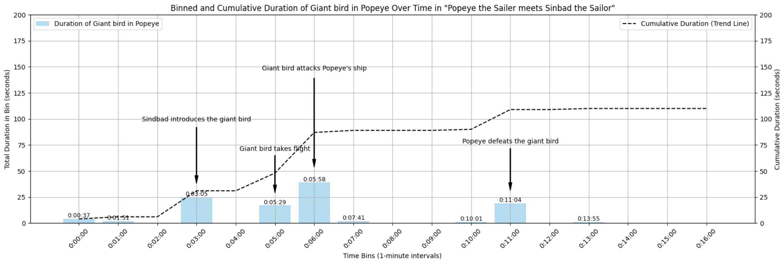
Updated over 1 year ago
Did this page help you?